My first Machine Learning model

In our last post we talked about what is Machine Learning and looked into its different categories of algorithms, as well as the most common algorithms in each of them. We saw that regression algorithms are one of the most common inside the Supervised Learning category, and that the simplest form of it was the linear regression. Because of its simplicity, this algorithm is often the first we get in touch when we start studying machine learning. It was no different with me, and I’ll share with you the steps I took until I was able to implement my first machine learning model!

What do you need to follow my steps?

To follow me in this process all you need is a desire to learn! I know it is a cliché, but really, you need just that. Of course, some linear algebra or calculus knowledge will help you understand better the theory behind the method, but what matters the most is to get intuition on what the method does, so you’re able to identify what’s the best method to solve your problem.

With that said, my goal is to give you this intuition without spending too much time in technical details. If you want to know more about the theory behind this method, feel free to reach out to me and I, as the passionate mathmatician that I am, will answer all your questions in detail!

For those who are curious, these are the details I do not intend to spend too much time on.

To implement the algorithm I decided to use Octave, a powerful free scientific software. Because it is a scientific software, Octave has most of the important functions and mathmatical operations we will need already programmed and heavily optimized, saving us the time to research, learn and import multiple libraries just so we can do some simple matrix operations. If you want to follow my implementation or to train the model by yourself using the code I’ll provide, you can download Octave here. For windows users, you can check a quick guide on how to install Octave here, on their Wiki.

It’s also important to note that the most used languages for machine learning are Python, R, JavaScript, Scala and Matlab/Octave. As I said above, Octave is a mathmatical software and, therefore, used the most for academic purposes. Python is probably the most popular programming language used for machine learning and I encourage you to look into it!

Finally, Linear Regression!

If you read the first article, you might remember that linear regression is used to model the relationship between two variables using a straight line. One way of measuring how well the model fits the original data is by calculating the average distance between our model and the entries of our dataset. This is often called as approximation error. An usual way of measuring this approximation error is through the mean squared error, which is basically the sum of the squared distancies between the model and the values from our dataset.

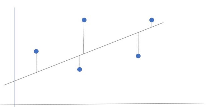
The distance between the set and the line is our approximation error.

The most important detail of this error measure is the fact that it is squared! Square functions have a very specific shape, with very good properties when the subject is maximizing or minimizing its value. As our goal here is to make our model fit the dataset as best as possible, we want to minimize the error. Here’s where Gradient Descent comes into play.

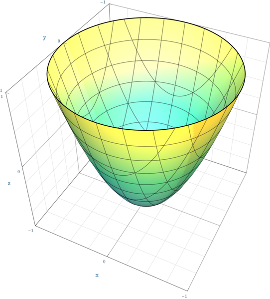
This is the figure formed by a 3D square function, a paraboloid!

Gradient Descent

As we saw, square functions have this bowl like shape that we call paraboloid. Just by looking at the figure we can see that its minimum is at its bottom, and there is exactly where gradient descent will lead us to!

Gradient descent is a simple, but versatile, method to solve minimization problems. In math, a gradient is a vector (some kind of an arrow) that points to the direction of greatest change in a function. Therefore, gradient descent is a method that will use the direction given by the gradient to lead us downhill until we find the funtions minimum. It’s like the function plot is a vert ramp and gradient descent put a skateboard at our feet, making us slide all the way down!

The downhill trajectory of a gradient descent.

The speed which we will slide in the gradients direction is called learning rate and it is generaly a constant value between 0 and 1. The secret of this method is to pick a good learning rate, because if we go down too fast we might end up climbing up the function on the other side and, in some cases, end up going up and down forever, never reaching the bottom.

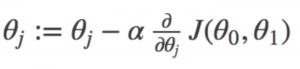
In the code I made the learning rate is the variable alpha (α). And speaking of code, lets get downt to business and see how gradient descent work by implementing it!

Getting down to business

Before we start, we need a problem to solve. I went to Kaggle and searched datasets fit to the application of regression and end up finding a really cool one with data from 100000 used cars for sale in UK, everything organised by car make and model. I ended up choosing the Ford Focus dataset, because it is a common car in Brazil, where I live.

The Kaggle dataset I chose.

Among the information found in this dataset, the price and mileage columns are the ones that caught my eye. We expect that cars with a bigger mileage would be cheaper, therefore we expect a correlation between mileage and price that we can estimate with regression.

The first step is to get a sample from the complete dataset, with more than 5000 entries, so we can train our model. I used some functions on the matrix I imported on Octave to extract a random sample with 500 entries. The next step, then, was to read this sample and prepare the data to be used in gradient descent.

data = csvread('data/focusSample.csv'); % Reads the sample file
data = sortrows(data,2); % Order data by mileage
prices = data(:,1); % Prices are found in the first column
mileage = data(:,2); % Mileage are found in the first column

To visualize the data we will use the scatter function, that draws a circle for each entry in our sample. The result should look like this:

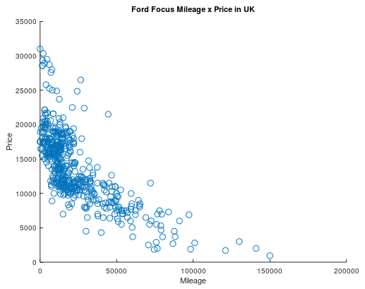
Each circle is an entry of our dataset, we are plotting price by mileage.

With that we confirmed our hypothesis that cars with a bigger mileage are, in general, cheaper. Now we must prepare our data to be used as input in the gradient descent. To achieve better performance with the algorithm it is ideal to have both variables in the same scale, so we will normalize both our variables. Normalizing is to divide the whole sample by its maximum value, making so that we only have values between 0 and 1 in it. We will also save these maximum so we can recover the original values later.

maxPrices = max(prices);
maxMileage = max(mileage);
prices = prices/maxPrices; % Normalize prices
mileage = mileage/maxMileage; % Normalize mileage

With the dataset ready, we will now focus on implementing our gradient descent. But before we start with its code, it’s important to remember the general equation for straight lines:

In it we see the dependent variable, y, the independent variable, x, and its coefficients, both θs (the greek letter theta). In our problem, y is the price of the car that we want to estimate using the mileage, x, by adjusting the θ coefficients. Finally, we will apply the gradient descent on θ and, to be able to directly use matrix operations, we will prepare our variables with the following:

alpha = 0.1; % Our learning rate
X = [ones(length(mileage), 1), mileage]; % matrix X, with [1, x]
y = prices; % target vector, with the prices from our sample
theta = zeros(2, 1); % we are using 0 as a initial guess for theta

Notice that we created a matrix X with two columns, the first is composed only by 1s and the second is the mileage from the training data. If you look at the general equation of straight lines we have 1 multiplying θ₀ and x, the mileage, multiplying θ₁. This is a pattern that can be extended for polynomials of any degree! For example, the code below would prepare a second degree polynomial to be used as input to our gradient descent:

X = [ones(length(mileage), 1), mileage, mileage.^2]; % now with x^2
y = prices;
theta = zeros(3, 1); % And we have 3 lines for theta

And now onwards to the promised gradient descent implementation! First we implement the cost function, that will estimate the approximation error at each iteration. This helped me a lot when I was investigating errors in the data or implementation of the model. This function is the sum of squared errors we discussed before:

With that done, the gradient descent implementation ended up like this:

Notice that I store, and return, the history of θ and the errors J. I did that so we can investigate any problems and also be able to plot our models evolution! So lets call this function and see how our model did:

[theta, cost_history, theta_history] = gradientDescent(X, y, theta, alpha, num_iters);
scatter(mileage*maxMileage,prices*maxPrices)
hold on
plot(X(:,2)*maxMileage,X*theta*maxPrices)
hold off

When you run the code above, a plot with the training data and our model will be shown. It will look like this:

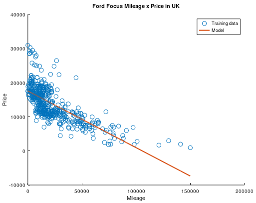
Not bad for our first model, right?

Even though it is not bad, our model is recommending negative resale values for cars with more than 100 thousand miles in its mileage, and that does not make sent, right? All in all, the squared mean error of our normalized model ended up being 0.026, which is far from ideal, but is not terrible for models of this kind.

What stood out, though, is that a straight line was not a good choice to model our data. When I started I noticed that the shape the training data assumed looked more like a square or exponential function than a straight line. Since this implementation is general enough to fit polynomials of any degree to a set of data, I decided to train a second degree polynomial to the same sample. This was the result:

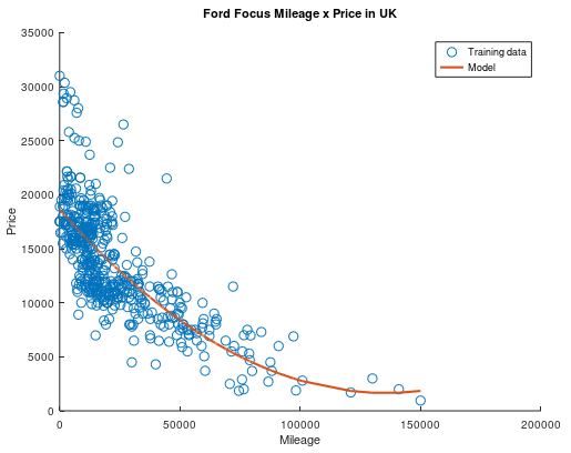
Much better, isn’t it?

Even though the square model is a much better fit at a first glance, the mean squared error is still 0.026 in the complete dataset. This can happen for a number of reasons, between them the learning rate or training sample choice, but this is a topic for a whole new article! While I learn about making better models, lets appreciate the evolution of our model during its training!

Beautiful, ain’t it?

Well, that’s it for today. I hope you enjoyed following my steps in the journey for my first machine learning model and, hopefully, learned something with me as well! Much of what I learned to write this post and build the model was taught in Andrew Ng’s machine learning course, feel free to check it out because it is worth it.

Lastly, stay tuned to our blog, because I want to share with you my journey to implement a Unsupervised Learning algorithm! Until then, I challenge you to get lower mean squared errors than the ones I got and, if you do, feel free to send me an email telling how you made it. The complete code I used is available on my GitHub, and the specific repository is found here!

See you soon!